: 磁性
: 輸送現象
: 不純物による散乱
目次
実際の導体の電気抵抗は温度とともに変化するが,この温度変化をする部分は伝導電子が格子振動(フォノン)によって散乱されることからおこる電気抵抗である.フォノンには振動の偏光方向や,音響型と光学型のタイプで区別される各モードにおいて振動数の分散があり,フォノンによる伝導電子の散乱は非弾性散乱である.
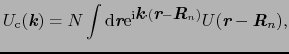
伝導電子に対するポテンシャル
 は結晶が完全に周期的に並んだときのものであり,それは
と書けるものとする.
 は
は 番目の原子からのポテンシャルである.格子点
 の原子が格子振動によって
 へ動いたとすると,そのための
の変化は
へ動いたとすると,そのための
の変化は
で与えられる.この が散乱ポテンシャル
 に相当する.いま伝導電子の波動関数を自由電子の関数に近似できるとすると
ここで
 |
|
|
(5.5.36) |
の記号を導入し,
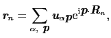
 をフォノンのモードで展開して
と表す. はモードを指定する添字である.
は実の量であるから
はモードを指定する添字である.
は実の量であるから
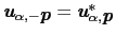 の関係が成り立つ.さらに
 を任意の逆格子ベクトルとして
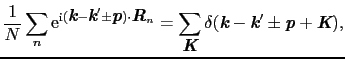 |
|
|
(5.5.37) |
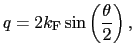
を用いると,(5.5.1)式は散乱ベクトル
 を使い,
を使い,
 |
|
|
(5.5.38) |
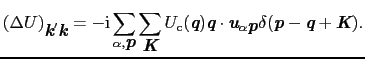
(5.5.4)式を(5.3.2)式に代入すれば,フォノンの散乱による
 への寄与が求まる.このときフォノンのモード
 の1次までの近似では,散乱過程でフォノンが吸収されるものと放出されるものがあり,(5.3.2)式におけるエネルギー保存則から
とおいて,
を満たすところが拾い出されるようになる.
 は波動ベクトル
 をもつフォノンのエネルギーである.
(5.5.4)式で
 の散乱過程を正常過程と呼び,
 のものをウムクラップ過程と呼ぶ.ウムクラップ過程では,
 の状態にある電子がフォノンとの散乱で
 の運動量だけでなく,結晶から
 の運動量をもらったり,与えたりする過程である.
ここでは正常過程だけを考える.すなわち(5.3.2)式の 関数におけるフォノンのエネルギー
を無視し,(5.5.4)式における
はゼロとおく.このときには(5.3.5)式を用いることができて,
関数におけるフォノンのエネルギー
を無視し,(5.5.4)式における
はゼロとおく.このときには(5.3.5)式を用いることができて,
 |
|
|
(5.5.39) |
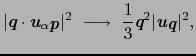
ここで
 は近似的に
は近似的に にあまり依存しないとして
 とおき,積分の外へ出せるとする.またフォノンの3つのモードを区別しない近似では
と書ける.
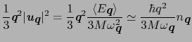
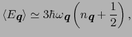
 で指定されたフォノンのエネルギーは運動エネルギーとポテンシャルエネルギーの和であるが,ビリアル定理により両者の統計的な平均値は等しいから,状態
のエネルギーの平均値は
で指定されたフォノンのエネルギーは運動エネルギーとポテンシャルエネルギーの和であるが,ビリアル定理により両者の統計的な平均値は等しいから,状態
のエネルギーの平均値は
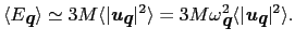 |
|
|
(5.5.40) |
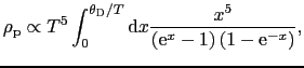
一方,フォノンはボーズ統計に従うので,分布関数
を使って,上のエネルギーは
 |
|
|
(5.5.41) |
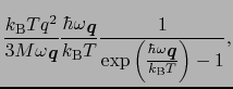
と表すこともできる.ここで の項はゼロ点エネルギーを表す項であり,これは電気抵抗に寄与しないので以下では無視する.(5.5.6)と(5.5.7)式から
が得られる.これを(5.5.5)式に代入して
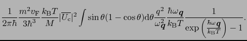
いまの弾性散乱の扱いでは,フォノンの波動ベクトル
に対しては
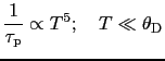
が成り立つ.さらにフォノンに対してはデバイ模型を仮定して
の関係式を用いると
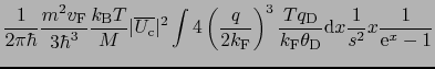
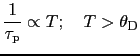
となる.この式から,
 では,0から
 の範囲のすべてのフォノンが熱的に励起されて積分に寄与するが,そのときの積分の上限
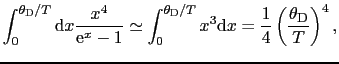
 は1に比べて小さいので,積分の中を
 で展開することが許される.その結果,
となり,
 |
|
|
(5.5.45) |
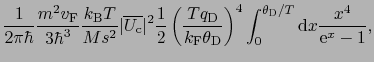
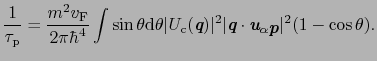
になることがわかる.一方
 であれば,積分の上限を
 で近似してよく,積分は
 に依らない値に近づくので,
 |
|
|
(5.5.46) |
になる.
以上はフォノンによる散乱を弾性散乱として扱った結果であるが,非弾性散乱の過程を正しく扱うと
 |
|
|
(5.5.47) |
という形の式が得られる.
: 磁性
: 輸送現象
: 不純物による散乱
目次
Masashige Onoda
平成18年4月7日
![$\displaystyle n_{\mbox{\bfseries\itshape {q}}} = \left[{\rm exp}\left(\frac{\hbar\omega_{\mbox{\bfseries\itshape {q}}}}{k_{\rm B}T}\right) - 1\right]^{-1},$](img763.png)
![$\displaystyle \sum_{n}\int{\rm d}\mbox{\bfseries\itshape {r}}{\rm e}^{-{\rm i}\...
...]{\rm e}^{{\rm i}\mbox{\bfseries\itshape {k}}\cdot\mbox{\bfseries\itshape {r}}}$](img735.png)
![$\displaystyle \sum_{n}\left[{\rm e}^{{\rm i}(\mbox{\bfseries\itshape {k}} - \mb...
...} - \mbox{\bfseries\itshape {R}}_{n} - \mbox{\bfseries\itshape {r}}_{n})\right]$](img736.png)
![$\displaystyle \sum_{n}\left[{\rm e}^{{\rm i}(\mbox{\bfseries\itshape {k}} - \mb...
...{n})}U(\mbox{\bfseries\itshape {r}} - \mbox{\bfseries\itshape {R}}_{n})\right].$](img737.png)