緩和時間

(5.2.1)式で導入した緩和時間$\tau$を量子力学的に考察してみよう．伝導電子が1つのブロッホ状態から他のブロッホ状態へ散乱されるのは，不純物や格子振動による格子の乱れによるのであり，その乱れは一般に自由度を含んでいる．格子振動の場合には，それはフォノンの振動数，進行方向，偏極の方向であり，不純物の場合であれば，その自由度は不純物にある電子の配置やスピンの向きである．伝導電子がこれらによって散乱されたときに，散乱体のエネルギー変化がなければ，その過程は弾性散乱であり，エネルギー変化のあるときは非弾性散乱と考えなければならない．

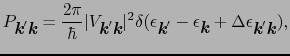
一般に摂動ポテンシャル$V$があるときに，系が $\vert\alpha\rangle$から$\vert\beta\rangle$へ移る遷移確率 $P_{\beta\alpha}$は，一次のボルン近似では

$$P_{\beta\alpha} = {2\pi \over{\hbar}}\vert V_{\beta\alpha}\vert^{2}\delta(E_{\beta} - E_{\alpha}),$$

で与えられる．伝導電子の $\vert\mbox{\bfseries\itshape {k}}\rangle$から $\vert\mbox{\bfseries\itshape {k}}'\rangle$への散乱に際して散乱体のエネルギー変化を $\Delta\epsilon_{\mbox{\bfseries\itshape {k}}'\mbox{\bfseries\itshape {k}}}$，散乱ポテンシャルを$V$とすると上式は

$$P_{\mbox{\bfseries\itshape {k}}'\mbox{\bfseries\itshape {k}}} = {... ... + \Delta\epsilon_{\mbox{\bfseries\itshape {k}}'\mbox{\bfseries\itshape {k}}}),$$ (5.3.18)

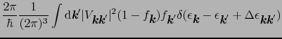
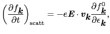
となる．散乱によって単位時間に $\vert\mbox{\bfseries\itshape {k}}\rangle$にある電子の分布の変化は，散乱でスピンは保存するとして，

$$\left({\partial f_{\mbox{\bfseries\itshape {k}}} \over{\partial t}}\right)_{\rm scatt} = {2\pi \over{\hbar}}{1 \over{(2\pi)^{3}}}\int{\rm d}\mbox{\bfserie... ...} + \Delta\epsilon_{\mbox{\bfseries\itshape {k}}\mbox{\bfseries\itshape {k}}'})$$

$$- {2\pi \over{\hbar}}{1 \over{(2\pi)^{3}}}\int{\rm d}\mbox{\bfserie... ... + \Delta\epsilon_{\mbox{\bfseries\itshape {k}}'\mbox{\bfseries\itshape {k}}}).$$ (5.3.19)

第1項は着目している $\vert\mbox{\bfseries\itshape {k}}\rangle$状態へ入ってくる散乱，第2項はそこから出て行く散乱を表す．

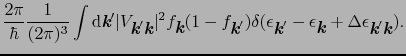
弾性散乱を考えることにして(5.3.2)式で $\Delta\epsilon_{\mbox{\bfseries\itshape {k}}\mbox{\bfseries\itshape {k}}'}$， $\Delta\epsilon_{\mbox{\bfseries\itshape {k}}'\mbox{\bfseries\itshape {k}}}$を無視しよう．

$$\left({\partial f_{\mbox{\bfseries\itshape {k}}} \over{\partial t... ...box{\bfseries\itshape {k}}'} - \epsilon_{\mbox{\bfseries\itshape {k}}})\right].$$

ここで(5.1.2)式を用いた．

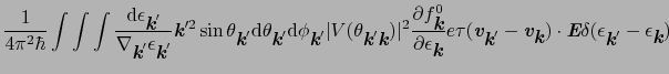
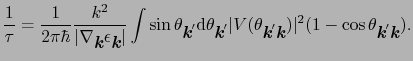
系は等方的であるとし， $V_{\mbox{\bfseries\itshape {k}}'\mbox{\bfseries\itshape {k}}}$は $\mbox{\bfseries\itshape {k}}$と $\mbox{\bfseries\itshape {k}}'$のなす角 $\theta_{\mbox{\bfseries\itshape {k}}'\mbox{\bfseries\itshape {k}}}$のみの関数とおく．いま仮定している緩和時間$\tau$を使って $g_{\mbox{\bfseries\itshape {k}}}$は(5.2.2)式で表されるから，

$$\left({\partial f_{\mbox{\bfseries\itshape {k}}} \over{\partial t}}\right)_{\rm scatt} = {1 \over{4\pi^{2}\hbar}}\int{\rm d}\mbox{\bfseries\itshape {k}}'\... ...ilon_{\mbox{\bfseries\itshape {k}}'} - \epsilon_{\mbox{\bfseries\itshape {k}}})$$

$$= {1 \over{4\pi^{2}\hbar}}\int{\rm d}\mbox{\bfseries\itshape {k}}'\... ...ilon_{\mbox{\bfseries\itshape {k}}'} - \epsilon_{\mbox{\bfseries\itshape {k}}})$$

$$= {1 \over{4\pi^{2}\hbar}}\int\int\int{{\rm d}\epsilon_{\mbox{\bfse... ...ilon_{\mbox{\bfseries\itshape {k}}'} - \epsilon_{\mbox{\bfseries\itshape {k}}})$$

$$= {1 \over{4\pi^{2}\hbar}}e\tau{\partial f^{0}_{\mbox{\bfseries\its... ...\itshape {v}}_{\mbox{\bfseries\itshape {k}}})\cdot\mbox{\bfseries\itshape {E}}.$$ (5.3.20)

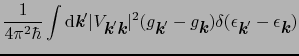
一方，(5.2.1)，(5.2.2)式より，

$$\left({\partial f_{\mbox{\bfseries\itshape {k}}} \over{\partial t... ...fseries\itshape {k}}} \over{\partial \epsilon_{\mbox{\bfseries\itshape {k}}}}},$$ (5.3.21)

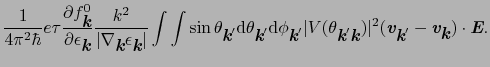
であるから，(5.3.3)，(5.3.4)式より

$$\left({\partial f_{\mbox{\bfseries\itshape {k}}} \over{\partial t... ...pe {k}}'\mbox{\bfseries\itshape {k}}})\right]\cdot\mbox{\bfseries\itshape {E}},$$

$${1 \over{\tau}} = {1 \over{2\pi\hbar}}{k^{2} \over{\vert\mbox{\bf... ...2}(1 - \cos\theta_{\mbox{\bfseries\itshape {k}}'\mbox{\bfseries\itshape {k}}}).$$ (5.3.22)

$\tau$は電気伝導のような輸送現象に特有の緩和時間である．

種々の散乱過程が存在するときには，それぞれの過程における散乱ポテンシャル$V$を求め，その散乱による緩和時間が上の式から得られるわけである．もしそれらが互いに独立な散乱過程であれば，それぞれの過程による緩和時間を$\tau_{\alpha}$として

$${1 \over{\tau}} = \sum_{\alpha}{1 \over{\tau_{\alpha}}},$$ (5.3.23)

で与えられる$\tau$が電気抵抗を決めることになる．